Cisco

Project description: This is a predictive analytics using the capital asset pricing model (CAPM) which is a simple asset pricing model in finance. CAPM is a linear regression model.

CAPM Explanation

Capital Asset Pricing Model (CAPM)

The capital asset pricing model (CAPM) is a simple asset pricing model in finance given by:

y_i = β₀ + β₁x_i + e_i

where y_i is a stock return and x_i is a market return at time i.

Some remarks are the following:

• β₁ measures the market-related (or systematic) risk of the stock.
• Market-related risk is unavoidable, while firm-specific risk may be 'diversified away' through hedging.
• Variance is a simple measure (and one of the most frequently-used) of risk in finance.

Capital Asset Pricing Model, CAPM

I applied the simple linear regression model to study the relationship between two series of financial returns – a regression of Cisco Systems stock returns, y, on S&P500 index returns, x (CAPM).

Stock returns are defined as:

return = (current price - previous price) / previous price ≈ log(current price / previous price)

when the difference between the two prices is small.

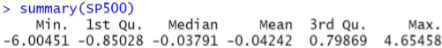
The data file ‘Returns.csv’ contains daily observations over a January - 29 December 2000 (i.e., n=252 returns). The dataset has 5 columns: Day, S&P500 return, Cisco return, Intel return and Sprint return.

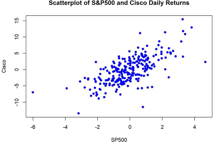
We can see that Cisco and S&P 500 is highly correlated which satisfies the assumption that the independent variable should be correlated with the dependent variable.

Capital Asset Pricing Model, CAPM

I fitted the regression model: Cisco = β₀ + β₁S&P500 + ε.

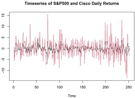
The rationale is that part of the fluctuation in Cisco returns was driven by the fluctuation in the S&P500 returns.

> reg <- lm(Cisco ~ SP500)
> summary(reg)

Call:
lm(formula = Cisco ~ SP500)

Coefficients:
            Estimate Std. Error t value Pr(>|t|)    
(Intercept)  -0.04547    0.19433   -0.234    0.815    
SP500         2.00715    0.13900   14.943   <2e-16 ***
---
Signif. codes:  0 ‘***’ 0.001 ‘**’ 0.01 ‘*’ 0.05 ‘.’ 0.1 ‘ ’ 1

Residual standard error: 3.083 on 205 degrees of freedom
Multiple R-squared: 0.4718, Adjusted R-squared: 0.4697
F-statistic: 223 on 1 and 204 DF, p-value: < 2.2e-16
    

Capital Asset Pricing Model (CAPM)

The estimated slope is β₁ = 2.07715. The null hypothesis H₀: β₁ = 0 is rejected with a p-value of 0.000 (to three decimal places). Therefore, the test is extremely significant.

The interpretation is that when the market index goes up by 1%, Cisco stock goes up by 2.07715%, on average. However, the error term ε in the model is large with an estimated σ_ε = 3.083%.

The p-value for testing H₀: β₀ = 0 is 0.815, so we cannot reject the hypothesis that β₀ = 0. Recall β₀ = y - β₁x and both y and ε are very close to 0.

R² = 47.18%, hence 47.18% of the variation of Cisco stock may be explained by the variation of the S&P 500 index, or, in other words, 47.18% of the risk in Cisco stock is the market-related risk.

1. Suggest hypotheses about the causes of observed phenomena

Part of the fluctuation in Cisco returns is driven by fluctuations in the S&P500 returns.

2. Assess assumptions on which statistical inference will be based

Based on the data and hypothesis that part of the fluctuation in Cisco returns is driven by fluctuations in the S&P500 returns, I made five(5) assumptions about the data and variables.

Linearity: The relationship between the predictor variable (S&P500) and the dependent variable (Cisco) is linear.

Scatter plot:

import matplotlib.pyplot as plt
plt.scatter(S&P500, Cisco)
plt.xlabel('Scatterplot of Stock and Market returns')
plt.ylabel('Cisco')
plt.show()

Residual plot: After fitting the regression model, plot residuals versus the fitted values.

plt.scatter(model.fittedvalues, model.residuals)
plt.xlabel('Fitted values')
plt.ylabel('Residuals')
plt.axhline(0, color='red', linestyle='--')
plt.show()

Independence: Observations are independent of each other.

Durbin-Watson Test

from statsmodels.stats.stattools import durbin_watson
dw = durbin_watson(model.residuals)
print(f'Durbin-Watson: {dw}')

Homoscedasticity: The variance of the residuals is constant across all levels of the predictor variable. This means there is no heteroscedasticity.

Residual Plot: I used the same residual plot to check if residuals have constant variance.

plt.scatter(model.fittedvalues, model.residuals)
plt.xlabel('Fitted values')
plt.ylabel('Residuals')
plt.axhline(0, color='red', linestyle='--')
plt.show()

Breusch-Pagan Test:

from statsmodels.compat import lzip
from statsmodels.stats.diagnostic import het_breuschpagan
test_stat, p_value, _, _ = het_breuschpagan(model.residuals, model.model.exog)
print(f'Breusch-Pagan test stat: {test_stat}, p-value: {p_value}')

Normality: The residuals are normally distributed.

Histogram of Residuals:

plt.hist(model.residuals, bins=30)
plt.show()

Q-Q Plot:

import statsmodels.api as sm
sm.qqplot(model.residuals, line='45')
plt.show()

Shapiro-Wilk Test:

from scipy.stats import shapiro
stat, p = shapiro(model.residuals)
print(f'Statistic={stat}, p-value={p}')

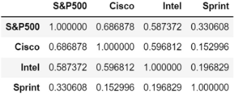
No Multicollinearity: The predictor variables are not highly correlated (if there are multiple predictors). But correlation between each predictor variable and the dependent variable should be high. That is correlation between S&P500, Intel and Sprint should be low but correlation between S&P500 and Cisco should be high.

Variance Inflation Factor (VIF):

from statsmodels.stats.outliers_influence import variance_inflation_factor
vif = [variance_inflation_factor(X.values, i) for i in range(X.shape[1])]
print(f'VIF: {vif}')

Correlation Matrix:

import seaborn as sns
corr_matrix = X.corr()
sns.heatmap(corr_matrix, annot=True)
plt.show()

3. Support the selection of appropriate statistical tools and techniques

Based on the hypothesis and assumptions, I selected linear regression as the statistical tool and technique which will be used to test whether part of the fluctuation in Cisco returns is explained by fluctuations in S&P500 returns. The dependent variable is Cisco returns and the predictor variable is S&P500.

4. Provide a basis for further data collection through surveys or experiments

Since the conclusion is that part (47%) of the fluctuations in Cisco returns is explained by fluctuations in S&P500 returns, a multiple linear regression can be used to test whether the remainder of the variation in Cisco returns is explained by earnings per share (EPS) and a price to earnings (P/E) ratio.

For more details see GitHub Flavored Markdown.